Ising Finite Size
In this post we’ll look at the finite size effect in the Ising model. We start by stating the energy of the Ising model,
$$ E = - J \sum_{\langle i, j\rangle} s_i sj - H \sum{i} s_i. $$
Where, $\langle i, j \rangle$ denotes the sum over nearest neighbour interactions. If we restrict ourselves to a square lattice with periodic boundary conditions we can compute this energy numerically as follows,
function energy(S)
    # J = 1, H = 0
    sum(- S .* (circshift(S, (1, 0)) .+ circshift(S, (0, 1))))
end
We would like to look at this system in equilibrium so we’ll need a method of sampling the equilibrium probability distribution. We can do this by constructing a Markov process that modifies the lattice one spin at a time and has an equilibrium distribution equal to our desired Boltzmann distribution.
This can be acheived using the Metropolis (Interestly, there is a fair amount of drama surrounding the origins of this algorithm. Details at Wikipedia’) algorithm for the transition rates for each spin.
$$ W(s \rightarrow s^\prime) = \min\left(1, e^{-\beta\Delta E(s, s^\prime)}\right) $$
We can consider one Markov step to be choosing a spin at random from the lattice and then flipping it with a probability consistent with the Metropolis transition frequency.
If we want to try flipping all the spins at once, we can do that too with a few caveats. If we use the Metropolis transition rates as they are currently presented we will quickly enter an oscillatory regime. To avoid that we can multiply the transition frequencies by a constant $\alpha $. This works because the detailed balance is maintained when we multiply both transition frequencies by the same constant.
$$ W(s \rightarrow s^\prime) = \min\left(\alpha, \alpha e^{-\beta\Delta E(s, s^\prime)}\right) $$
# Flip a spin with the modified Metropolis rate
function flip(s, ΔE, β)
    # α = 0.3
    if ΔE < 0
        rand() < 0.3 ? (return -s) : (return s)
    else
        rand() < 0.3 * exp(- β * ΔE) ? (return -s) :
            (return s)
    end
end

# Step Lattice one Markov step forward in "time"
function step!(S, β)
    ΔE = 2. * S .* (circshift(S, (0, 1)) .+
                   circshift(S, (0, -1)) .+
                   circshift(S, (1, 0)) .+
                   circshift(S, (-1, 0)))

    for i in eachindex(S)
        S[i] = flip(S[i], ΔE[i], β)
    end
    return
end
Measuring Equilibrium Statistics
Now we’d like to measure equilibrium statistics across a variety of temperatures. If we start with the very high temperatures with an initial condition that is random we won’t need to wait long for the Markov process to equilibrate before we start to sample.
First we need a method to compute energy statistics at a single temperature though.
function energy_stats(S, β; samples = 100)
    # Mean and variance of the energy at temperature β

    energies = Float64[]

    for sample in 1:samples
        step!(S, β)
        push!(energies, energy(S))
    end

    meanE = mean(energies)
    varE = mean((i - meanE)^2 for i in energies)

    return meanE / length(S), varE / length(S)
end
Now we can make a function to do a temperature sweep for lattices of a given size over a particular temperature range
function sweep(N, Trange; smpl_per_temp=100)

    Trange = reverse(Trange)

    S = rand([1.0, -1.0], (N, N))
    means = Float64[]
    vars = Float64[]

    for (i, T) in enumerate(Trange)
        m, v = energy_stats(S, T^(-1), samples=smpl_per_temp)
        push!(means, m)
        push!(vars, v)
    end

    return reverse(means), reverse(vars)
end
Visualization
Ok, now that we’ve got all the technical details out of the way lets brew up some visualization so we can make sure things are working as we might expect. Unicode is a great asset here.
With a pretty printing function pprint in hand lets do a little animation to
see things are working.
function pprint(S)
    N, M = size(S)
    for i in 1:N
        for j in 1:M
            S[i, j] > 0 ? print("⬛") : print("⬜")
        end
        print("\n")
    end
end

# In a Jupyter notebook we can make
# a small animation in the output cell
using IJulia

S = rand([1.0, -1.0], (20, 20))
T = 3.0

for i in 1:40

    step!(S, 1.0/T)
    IJulia.clear_output(true)
    pprint(S)

    sleep(0.1)
end
⬛⬛⬜⬜⬜⬜⬛⬛⬛⬜⬜⬜⬜⬜⬛⬜⬜⬜⬜⬛ ⬛⬜⬛⬜⬛⬛⬛⬛⬜⬛⬛⬜⬜⬜⬜⬜⬜⬜⬜⬜ ⬛⬜⬜⬜⬜⬜⬜⬜⬛⬛⬛⬛⬜⬜⬛⬛⬜⬜⬜⬜ ⬜⬛⬜⬜⬜⬜⬜⬜⬛⬛⬛⬛⬛⬛⬛⬛⬜⬜⬜⬜ ⬜⬛⬜⬜⬛⬛⬛⬜⬛⬛⬛⬜⬛⬛⬜⬜⬛⬛⬜⬜ ⬜⬜⬜⬜⬜⬜⬛⬛⬜⬛⬛⬜⬛⬛⬜⬛⬛⬜⬜⬜ ⬜⬛⬜⬜⬜⬜⬛⬛⬛⬛⬜⬜⬛⬜⬜⬛⬜⬛⬜⬜ ⬜⬜⬜⬜⬜⬛⬛⬛⬛⬛⬜⬜⬜⬜⬛⬛⬛⬛⬜⬛ ⬜⬜⬜⬜⬜⬜⬛⬛⬛⬜⬜⬜⬛⬜⬛⬛⬛⬛⬜⬛ ⬜⬜⬜⬜⬜⬜⬜⬛⬛⬛⬛⬛⬜⬛⬛⬛⬜⬜⬜⬜ ⬜⬜⬜⬜⬛⬛⬜⬛⬜⬛⬛⬜⬛⬜⬜⬜⬜⬜⬜⬛ ⬜⬜⬜⬜⬛⬛⬛⬜⬜⬜⬜⬜⬛⬜⬜⬜⬛⬛⬛⬛ ⬜⬜⬜⬜⬜⬜⬛⬛⬜⬜⬜⬜⬛⬜⬛⬛⬜⬛⬜⬜ ⬜⬛⬜⬜⬛⬜⬛⬛⬛⬛⬛⬜⬜⬛⬜⬜⬜⬜⬜⬜ ⬜⬛⬜⬛⬛⬜⬜⬜⬜⬜⬛⬛⬜⬛⬜⬜⬜⬜⬜⬛ ⬛⬛⬛⬛⬛⬜⬛⬜⬛⬛⬜⬛⬜⬜⬜⬜⬜⬜⬜⬛ ⬛⬛⬛⬛⬜⬛⬜⬛⬛⬛⬜⬜⬜⬜⬛⬛⬜⬜⬜⬛ ⬛⬛⬜⬛⬜⬜⬜⬛⬛⬛⬜⬛⬜⬛⬛⬛⬛⬜⬛⬛ ⬛⬛⬛⬛⬜⬜⬜⬜⬜⬛⬛⬜⬛⬜⬛⬜⬜⬜⬛⬛ ⬛⬛⬛⬛⬜⬛⬜⬛⬜⬜⬜⬛⬜⬛⬛⬜⬜⬛⬛⬛
Lovely! Lets get some results then!
# Perform a sweep to check for phase transition
T = 1.0:0.05:4.0
means, vars = sweep(20, T, smpl_per_temp=20000)
# Cᵥ = (kb*T²)⁻¹⟨ΔE²⟩
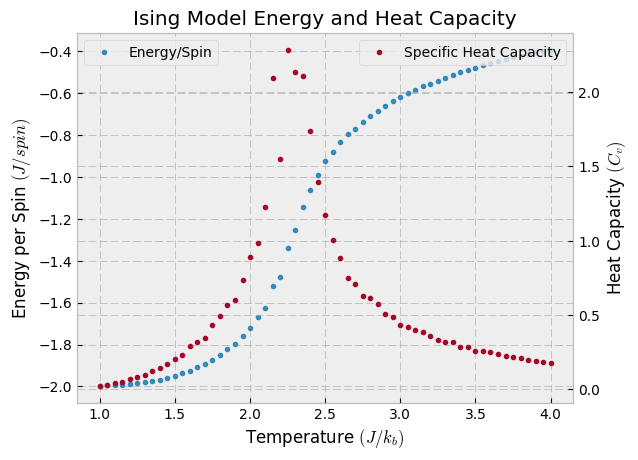
Cᵥ = vars ./ T.^2;$ C_v(T) $ and $ E(T) $ Results
Performing a temperature sweep on a 20 x 20 lattice with 20000 samples per temperature, we see the characteristic divergence of the heat capacity around $ T_c $. Note that the theoretical result for $ T_c $ in the thermodynamic limit is,
$$ T_c = \frac{2}{\ln\left(2 + \sqrt{2}\right)} \approx 2.2691… $$
The key question here is, how accurate are those results? While we know the theoretical solution in the case of the 2D Ising model, in more general circumstances we need to ask: how do we know if the answer has converged? The answer, as per usual, is in the limit. As we examine larger and larger lattices, we look for convergence in the solution.
# Sweep of lattices sizes from 2 -> 48
sizes = [2, 4, 8, 16, 24, 48]
smpls = [30000, 30000, 10000, 10000, 5000, 1000]
T = 1.0:0.05:4.0

for (size, smpl) in zip(sizes, smpls)
    mean, _ = sweep(size, T, smpl_per_temp=smpl)
    IJulia.clear_output(true)
    println("Done size $size")
    plot(T, mean, label="$size × $size")
end

legend()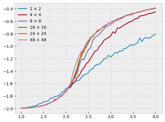
Summary
Finite size systems are different than their infinite counterparts. Its important to remember that numerical techniques are always limited in their ability to approximate the thermodynamic limit. We haven’t really broached the subject of absolute convergence here, but at least in relative way we can see convergence for numerical methods by comparing results for larger and larger systems.